40 add data labels to pivot chart
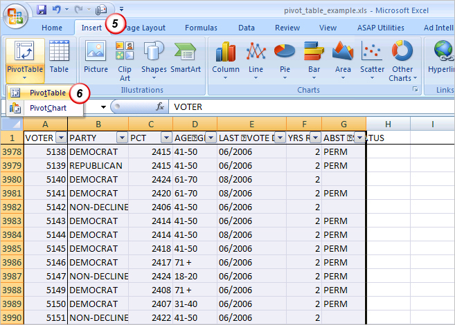
Automatic Row And Column Pivot Table Labels Select the data set you want to use for your table The first thing to do is put your cursor somewhere in your data list Select the Insert Tab Hit Pivot Table icon Next select Pivot Table option Select a table or range option Select to put your Table on a New Worksheet or on the current one, for this tutorial select the first option Click Ok How do I add a column of data in a pivot table ... How do I add a column of data in a pivot table? Add an Additional Row or Column Field. Click any cell in the PivotTable. The PivotTable Fields pane appears. You can also turn on the PivotTable Fields pane by clicking the Field List button on the Analyze tab. Click and drag a field to the Rows or Columns area.
How to add data labels from different column in an Excel ... Right click the data series in the chart, and select Add Data Labels > Add Data Labels from the context menu to add data labels. 2. Click any data label to select all data labels, and then click the specified data label to select it only in the chart. 3.

Add data labels to pivot chart
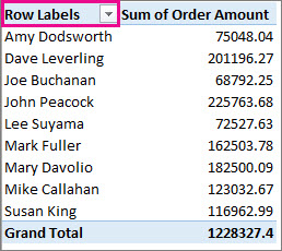
How to update or add new data to an existing Pivot Table ... Change the Source Data for your Pivot Table In order to change the source data for your Pivot Table, you can follow these steps: Add your new data to the existing data table. In our case, we'll simply paste the additional rows of data into the existing sales data table. Here's a shot of some of our additional data. Add the count of data to data labels to a pivot chart in excel You need to add the 'Data Labels' first for all lines. Then go to individual data labels & refer it to the cell you need by selecting one label at a time and press "=". Every time the data in the reference cells change, the data labels change too. I have updated the data labels in the attached file. Attached Images Pivot table row labels side by side - Excel Tutorials 3. Now, let's create a pivot table ( Insert >> Tables >> Pivot Table) and check all the values in Pivot Table Fields. Fields should look like this. Right-click inside a pivot table and choose PivotTable Options…. Check data as shown on the image below. The table is going to change. The pivot table is almost ready.
Add data labels to pivot chart. How to Add Data to a Pivot Table: 11 Steps (with Pictures) Open your pivot table Excel document. Double-click the Excel document that contains your pivot table. It will open. Go to the spreadsheet page that contains your data. Click the tab that contains your data (e.g., Sheet 2) at the bottom of the Excel window. Add or change your data. Enter the data that you want to add to your pivot table directly ... Excel charts: add title, customize chart axis, legend and ... Click the data series you want to label. To add a label to one data point, click that data point after selecting the series. Click the Chart Elements button, and select the Data Labels option. For example, this is how we can add labels to one of the data series in our Excel chart: Add a DATA LABEL to ONE POINT on a chart in Excel Steps shown in the video above: Click on the chart line to add the data point to. All the data points will be highlighted. Click again on the single point that you want to add a data label to. Right-click and select ' Add data label ' This is the key step! Right-click again on the data point itself (not the label) and select ' Format data label '. How to add Data label in Stacked column chart of Pivot charts Show activity on this post. I'm tring to make a Pivot chart with stacked column graph. In where, i couldn't add data label for cumulative sum of value in Data label. Where i could only add data label to individual stacks in column graph. It found possible with normal stacked column chart without pivot chart.
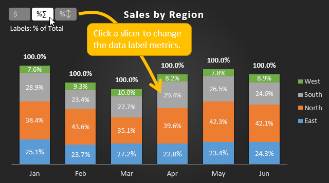
How to Customize Your Excel Pivot Chart Data Labels - dummies To add data labels, just select the command that corresponds to the location you want. To remove the labels, select the None command. If you want to specify what Excel should use for the data label, choose the More Data Labels Options command from the Data Labels menu. Excel displays the Format Data Labels pane. Create Dynamic Chart Data Labels with Slicers - Excel Campus You basically need to select a label series, then press the Value from Cells button in the Format Data Labels menu. Then select the range that contains the metrics for that series. Click to Enlarge Repeat this step for each series in the chart. If you are using Excel 2010 or earlier the chart will look like the following when you open the file. Include Grand Totals in Pivot Charts - My Online Training Hub Step 5: Format the Chart. The Grand Total value is the top segment of the stacked column chart. We need to hide this, but first let's select the grand total series and add Data Labels > Inside Base: Next, with the grand total series still selected go to the Format tab > Shape Fill > No Fill. Hide the gridlines and vertical axis, and place the ... How to Customize Your Excel Pivot Chart and Axis Titles The Chart Title and Axis Titles commands, which appear when you click the Design tab's Add Chart Elements command button in Excel, let you add a title to your chart titles to the vertical, horizontal, and depth axes of your chart. In Excel 2007 and Excel 2010, you use the Chart Title and Axis Titles commands on the Layout tab to add chart and axis titles. After you choose the Chart ...
Add a data label on Pivot Chart With .SeriesCollection (1).Points (i) .HasDataLabel = True .DataLabel.Text = Worksheets ("Sheet2").Range ("a" & position_total).Value position_total = position_total + 1 End With End With Next End Sub Select the Pivot chart, then run the macro "data_label". Jaynet Zhang TechNet Community Support Add a Data Callout Label to Charts in Excel 2013 The new Data Callout Labels make it easier to show the details about the data series or its individual data points in a clear and easy to read format. How to Add a Data Callout Label. Click on the data series or chart. In the upper right corner, next to your chart, click the Chart Elements button (plus sign), and then click Data Labels. Formal ALL data labels in a pivot chart at once ... How do I format all data labels for all series in a chart at once? I frequently make pivot charts with multiple data series (line graphs). I know how to click on a data point and use the pane on the right to format the labels for that series, but it only changes that series. Add or remove data labels in a chart - support.microsoft.com To label one data point, after clicking the series, click that data point. In the upper right corner, next to the chart, click Add Chart Element > Data Labels. To change the location, click the arrow, and choose an option. If you want to show your data label inside a text bubble shape, click Data Callout.
excel - remove data labels automatically for new columns in pivot chart? - Stack Overflow
How to make row labels on same line in pivot table? Make row labels on same line with PivotTable Options You can also go to the PivotTable Options dialog box to set an option to finish this operation. 1. Click any one cell in the pivot table, and right click to choose PivotTable Options, see screenshot: 2.

How to Sort Pivot Table Row Labels, Column Field Labels and Data Values with Excel VBA Macro ...
Adding Data Labels to a Chart Using VBA Loops - Wise Owl To do this, add the following line to your code: 'make sure data labels are turned on. FilmDataSeries.HasDataLabels = True. This simple bit of code uses the variable we set earlier to turn on the data labels for the chart. Without this line, when we try to set the text of the first data label our code would fall over.
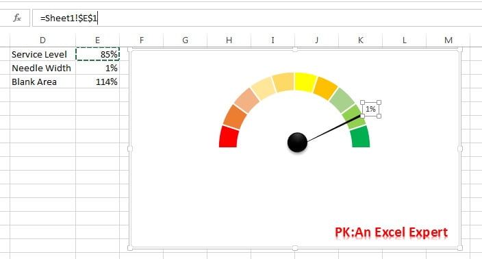
Speedometer Chart - PK: An Excel Expert
Adding rich data labels to charts in Excel 2013 ... To add a data label in a shape, select the data point of interest, then right-click it to pull up the context menu. Click Add Data Label, then click Add Data Callout . The result is that your data label will appear in a graphical callout. In this case, the category Thr for the particular data label is automatically added to the callout too.

How to Create Multi-Category Chart in Excel - Excel Board
How to add data labels to pivot chart? | Console App ... The CSV data goes into the Data sheet and the application then creates a pivot table and corresponding pivot chart from this data in the Charts sheet. The chart is created alright but i see no option to add data labels to it using XlsIO. The chart is created as follows: IChartShape pivotChart = chartsSheet.Charts.Add();

Did you know: Multiple Pivot Charts for the SAME pivot table? - Efficiency 365
Change the format of data labels in a chart To get there, after adding your data labels, select the data label to format, and then click Chart Elements > Data Labels > More Options. To go to the appropriate area, click one of the four icons ( Fill & Line, Effects, Size & Properties ( Layout & Properties in Outlook or Word), or Label Options) shown here.
Sort data in a PivotTable or PivotChart
Add data and format Pivot Chart using VBA Excel - Stack ... I am struggling to format a Pivotchart & add data to the chart using VBA. I have setup the code to create the pivot chart which is working fine and I can manually format & add data but when... Stack Overflow ... which I assume is causing an issue since you're adding to a chart, not the pivot cache.

WinForms Pivot Chart Control | Business Charts | Syncfusion
Add Value Label to Pivot Chart Displayed as Percentage If you use the hidden line method: How to Add Total Data Labels to the Excel Stacked Bar Chart and then use the code mentioned in post #2 to create boxes offset from the hidden line points, you should be able to place the additional labels where you want. You must log in or register to reply here. Similar threads E

excel - How can I incorporate a PivotTable right into the source data on the sheet (using EPPlus ...
Pivot table row labels side by side - Excel Tutorials 3. Now, let's create a pivot table ( Insert >> Tables >> Pivot Table) and check all the values in Pivot Table Fields. Fields should look like this. Right-click inside a pivot table and choose PivotTable Options…. Check data as shown on the image below. The table is going to change. The pivot table is almost ready.
Create Dynamic Chart Data Labels with Slicers - Excel Campus
Add the count of data to data labels to a pivot chart in excel You need to add the 'Data Labels' first for all lines. Then go to individual data labels & refer it to the cell you need by selecting one label at a time and press "=". Every time the data in the reference cells change, the data labels change too. I have updated the data labels in the attached file. Attached Images

31 Excel Chart Label Axis - Label Design Ideas 2020
How to update or add new data to an existing Pivot Table ... Change the Source Data for your Pivot Table In order to change the source data for your Pivot Table, you can follow these steps: Add your new data to the existing data table. In our case, we'll simply paste the additional rows of data into the existing sales data table. Here's a shot of some of our additional data.
In Search of the Elusive Pivot Table | Dynamic Edge, Inc. | Beyond Tech Support Dynamic Edge ...
How to add the average baseline for a specific pivot chart | Dashboards & Charts | Excel Forum ...

vba - Pie Chart - Move Data Labels off Chart - Stack Overflow

excel vba - VBA Pivot Chart data labels not appear - Stack Overflow
Post a Comment for "40 add data labels to pivot chart"